YOLO: Real-Time Object Detection Explained

If you’ve read the Haar cascade theory post on this blog, you already know one way to find objects in an image: slide a small window across the picture at many scales and positions, and ask a classifier “is this a face?” at every single stop. It works, but it is fundamentally a search problem — you are hunting for the object patch by patch.

YOLO (“You Only Look Once”) throws that idea out. Instead of scanning the image hundreds or thousands of times, YOLO looks at the entire image once, in a single forward pass through a neural network, and directly predicts every object’s location and class at the same time. That single design choice is why YOLO can run at real-time video speeds while classic sliding-window detectors struggle.

Why sliding windows are slow

A sliding-window detector like Viola-Jones (Haar cascades) has to:

1. Slide a fixed-size window over the image.
2. Resize the window (or the image) to check for objects at different scales.
3. Run a classifier on every single window position.

Even with tricks like cascading classifiers to reject non-faces early, this is still thousands of small classification calls per image. It’s fine for a narrow task like frontal face detection, but it doesn’t scale well to detecting dozens of object classes at arbitrary sizes and positions.

How YOLO’s single pass works

YOLO reframes detection as a regression problem rather than a classification-per-window problem. Here is the conceptual pipeline:

1. Grid the image. YOLO divides the input image into an S×S grid of cells (e.g., 13×13 or 19×19 depending on the version and input resolution).
2. Each cell makes predictions. Every grid cell predicts a fixed number of bounding boxes, each with:
   • x, y, w, h — the box’s center coordinates and size, relative to the cell.
   • a confidence score — how sure the model is that an object exists in that box.
   • a class probability distribution — what the object most likely is (car, person, dog, …).
3. One forward pass, one big tensor out. All of this — for every cell and every box — is produced by a single convolutional neural network in one shot. There is no cropping, resizing, and re-running the network per region.
4. Non-max suppression cleans up. Because neighboring cells often each propose a box for the same object, a post-processing step called non-max suppression (NMS) discards overlapping, lower-confidence boxes and keeps the best one per object.

The network is trained end-to-end on labeled images with bounding boxes, so it directly learns to associate visual patterns with “there is an object here, this is roughly its shape, and this is what it probably is.” Later versions of YOLO (v3 through v8/v11 and beyond) refined this with multi-scale prediction grids, anchor boxes or anchor-free heads, better backbones, and improved loss functions — but the “look once, predict everything at once” core idea stays the same.

Why this makes YOLO fast

• One network pass per image instead of thousands of classifier evaluations.
• Global context. Because the whole image is processed at once, the model implicitly sees the relationships between objects and the background, which also helps reduce false positives compared to a window that only sees a small crop.
• GPU-friendly. A single large convolutional pass parallelizes extremely well on modern hardware, which is exactly why YOLO models can hit 30-100+ frames per second on real-time video, something a per-window Haar cascade or an R-CNN-style “propose regions, then classify each one” pipeline cannot easily match.

The trade-off: YOLO can struggle a bit more with very small or tightly packed objects compared to slower, two-stage detectors, since each grid cell is only responsible for a limited number of boxes. Modern versions have largely closed this gap with better multi-scale detection heads.

A minimal working example

Using the popular ultralytics package (which implements modern YOLO versions), running detection on an image takes only a few lines:

pip install ultralytics

from ultralytics import YOLO

# Load a small pretrained model (trained on the COCO dataset, 80 classes)
model = YOLO("yolov8n.pt")

# Run detection on an image
results = model("street_scene.jpg")

# Print detected classes, confidence scores, and box coordinates
for r in results:
    for box in r.boxes:
        cls_id = int(box.cls[0])
        conf = float(box.conf[0])
        xyxy = box.xyxy[0].tolist()
        print(f"{model.names[cls_id]}: {conf:.2f} at {xyxy}")

# Save the image with bounding boxes drawn on it
results[0].save(filename="street_scene_detected.jpg")

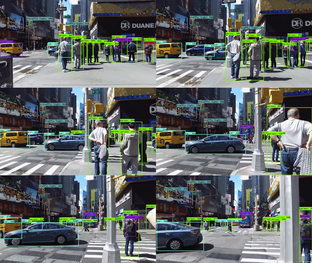
That’s it — no manual sliding window, no hand-picked Haar features, no threshold tuning per image. The model was pretrained on the COCO dataset, so out of the box it already recognizes 80 everyday object classes like person, car, and traffic light — the same kind of scene you’d see in the bounding-box image above.

Where YOLO fits versus Haar cascades

If you’re deciding which approach to reach for:

• Haar cascades are lightweight, extremely fast to run on very limited hardware, and good for a single, narrow, well-defined object class (classic use case: frontal faces). See the Haar cascade theory and practical OpenCV implementation posts on this blog.
• YOLO is the better default for general-purpose, multi-class, real-time object detection — self-driving cars, video surveillance, retail analytics, robotics — anywhere you need to detect many kinds of objects at once, quickly, from a single model.

For a broader primer on how computer vision represents and processes images in the first place, check out Know About Computer Vision.

Made with ❤️ by Vaibhav Hariramani